Transmission Line Reflection Coefficient

This article sets out to illustrate a numerical example of a mismatched transmission line and, along the way, uncover the derivation and use of the reflection coefficient. I’m hoping that it will also serve as a reference to come back to the next time you need to calculate reflected voltages or currents. I have often scratched my head trying to recall how to do these calculations. In my impatience, I’ve searched for internet articles showing, for instance, bounce diagrams or oscilloscope captures that, in the end, proved to be ambiguous. I hope this article will provide a clearer picture. I’m also going to show you how modern-day simulation tools can solve this problem and give you the answers you need. Still, you also will benefit from understanding the math behind the simulation results.
A Basic Circuit Example of Transmission Line Reflection Coefficient
A 12-volt source connects to a 24 Ω load via a cable with a 50 Ω characteristic impedance (Z0). A short time later, 12 volts arrive at the load accompanied by a current of 240 mA (12 volts 50 Ω). But, because the load is 24 Ω, there is a potential violation of Ohm’s law. To resolve this disparity, the 12 volts need to be reduced, and the 240 mA needs to be increased so that they adopt the correct 24 Ω ratio. It’s all about fixing the violation.
Imagining a Different Result With no Violation
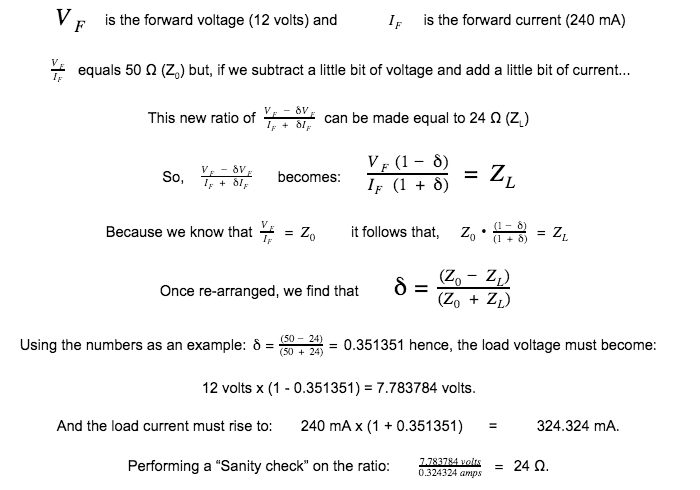
This tells us what the end-game looks like, but not how it is achieved.
Reaching a Result That Doesn’t Violate Ohm’s Law
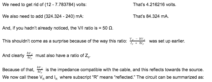
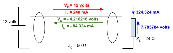
VR is negative because the load impedance is lower, so by Ohm's law the voltage drop across the load is lower. IR is also negative because (a) it has to be the same polarity as VR to match Z0 = 50 Ω, while (b) flows backward with a negative sign, which has the same effect as flowing forward with a positive value.
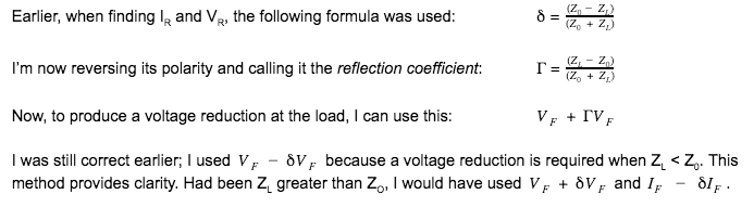
A Small Change in Terminology
What Happens Next?
The initial load reflections have now arrived at the source and, to move forward, we should consider the reflection coefficient equation at the source:

Because the source is directly connected in this example, ZS = 0 Ω, and hence 𝛤S = -1. This should illustrate why we might use a series resistor at the source: it provides impedance matching at the source and sets 𝛤 = 0.
The initial source-bound load-reflection of -4.216216 volts becomes a load-bound source-reflection of +4.216216 volts accompanied by a current of +84.324 mA (due to Z0). This adds to the load-bound current, i.e., 324.324 mA becomes 408.648 mA in the direction of the load.
There are a couple approximations to note about these equations:
- Driver's output impedance: I've defined the output impedance as ZS = 0 Ω on the source side, but this is not really true. The output impedance of CMOS buffer drivers and other logic families is less than the common 50 Ohm standard, but it's not zero. We just use ZS = 0 Ω as an approximation.
- Line's input impedance: The line is assumed to be electrically long, meaning the input impedance of the line converges to the transmission line characteristic impedance.
Most textbooks and design guides won't tell you these points, and you'll be left to figure them out on your own. We'll stick with these approximation as it's still useful to see what happens when there is total reflection off the source end. This creates the back-and-forth oscillation of signal that we'll see in the simulation below.
A Simple Simulation Can Help
The following simulation looks at three points. VIN (red) is the source level of 12 volts. VMID (green) is at the mid-point of the cable, and VOUT (blue) is across the 24 Ω load. At t = 0 ns, 12 volts is applied. In this simple simulation, we're assuming the input pulse rises instantly to its final value. The speed of the signal can be read out as the delay between the red line and the green line.
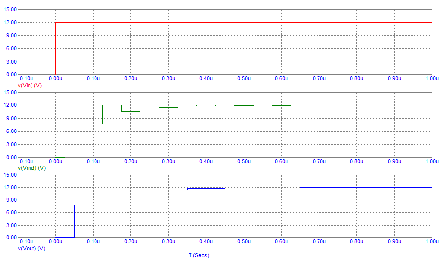
At t = 25 ns, VMID registers a level of 12 volts. This is the applied voltage traveling down the cable.
At t = 50 ns, VOUT is 7.783784 volts. This is the applied 12 volts minus the reflection of 4.216216 volts.
At t = 75 ns VMID registers the source-bound load-reflection - it falls to 7.783784 volts from 12 volts.
At t = 100 ns, the source impedance (0 Ω) starts modifying the incoming -4.216216 volts from the load into a load-bound reflection of +4.216216 volts. This adds to the prevailing 7.783784 volts.
At t = 125 ns, 12 volts is seen at the cable mid-point (7.783784 volts plus 4.216216 volts).
At t = 150 ns, we witness the 2nd occurrence of a load reflection but, instead of the original 12-volt step traveling down the cable to the source, the step is now only +4.216216 volts, and only that step voltage is subject to modification by the transmission line reflection coefficient at the load, 𝛤L.
At t = 150 ns, the voltage now seen at the load is 10.518627 volts. This naturally produces a load current into 24 Ω of 438.275 mA, but how do we account for the new voltage and current?
It’s probably worth looking at the currents that are flowing in the transmission line, load, and source to help with our understanding:
At t = 25 ns, IMID is a current of 240 mA. This is traveling down the cable, and 240 mA is 12 volts50 Ω.
At t = 50 ns, ILOAD becomes 324.324 mA. This is the applied 240 mA plus the reflection of -84.324 mA. Remember that a negative reflection current adds to the forward current. From the voltage level simulation, 7.783784 volts0.324324 amps = 24 Ω.
At t = 75 ns, IMID becomes a current of 324.324 mA. This is the summing of the forward current of 240 mA and the reflected current of -84.324 mA.
At t = 100 ns, ISOURCE becomes 408.649 mA. This is the original 240 mA plus the initial reflection of 84.324 mA, now being increased by another load-bound (forward traveling) current of 84.324 mA.
At t = 125 ns, IMID becomes a current of 408.648 mA.
At t = 150 ns, ILOAD becomes 438.275 mA, i.e., 324.324 mA is increased by 113.951 mA. The extra current arises from the latest load-bound current of 84.324 mA being reflected and reversed by 𝛤S = -0.351351. We can see that 1.351351 x 84.324 mA = 113.951 mA.
It might be becoming somewhat apparent that keeping track of the evolving changes is tricky.
Conclusions
So, should I (or indeed anyone) persevere in running through the never-ending but ever-decreasing transmission line reflection scenarios? I don’t think I need to because the main object of this article is to show the reasoning behind the presence of voltage and current reflections and, hopefully, that has been accomplished. My reasoning is summarized below:
- The source current that initially flows down a cable towards a load is governed only by the cable’s characteristic impedance and the source voltage (Ohm’s law).
- When there is a mismatch of load and cable impedance, there appears to be a potential violation of Ohm’s law, and, of course, this must be resolved or explained.
- When the load impedance is smaller than the cable’s impedance, the voltage arriving at the load has to be reduced, AND the current needs to be increased so that Ohm’s law is not violated.
- If the load impedance is larger than the cable’s impedance, the voltage arriving at the load has to be increased, AND the current needs to be decreased so that Ohm’s law is not violated.
- In resolving the potential violation, we find that the necessary voltage and current changes will naturally have a ΔVΔI ratio that completely matches the cable’s characteristic impedance (Z0).
- This means that those “unwanted” (or excessive) current and voltage changes find a natural “escape route” by using the cable itself. This is called a “reflection” and complies with Ohm’s law entirely.
Of secondary importance (but still very important) is recognizing the near-futility in the labor-intensive calculations needed to find the reflected voltages and currents. Compare the hand-made methods against a modern simulation tool as I have shown above. Sure, if all you had was a simulation tool producing the above plots, you probably wouldn’t be able to figure out what was going on. So, the third reason for creating this document is to show a worked numerical example that, along the way, explains and derives the transmission line reflection coefficient.
Have more questions? Call an expert at Altium and discover how we can help you with your next PCB design.